Line Chart & small multiple
Small multiple is a dataviz technique allowing to study several groups on the same figure. Repeating all groups but faded out adds some useful context to each section.
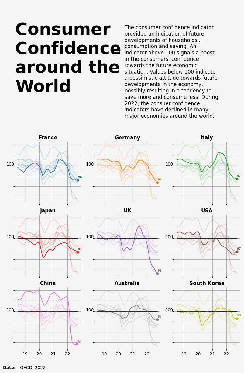
This plot is a small multiple Line Chart, initially published in the Visual Capitalist. It shows the evolution of a metric (the consumer confidence around the world) in the last few years. Each item of the small multiple provides the evolution of a specific country.
Interestingly, all other countries are displayed too, but nicely faded out. As a retult, the evolution of the target country is obvious, and it’s possible to put it in perspective with other countries.
Libraries
We need to install the following librairies:
- matplotlib is used for creating the chart and add customization features
pandasis used to put the data into a dataframedatetimeis used for dealing with the date format of our time variable
# !pip install matplotlib pandas numpy

import matplotlib.pyplot as plt
import pandas as pd
import datetime
Dataset
For this reproduction, we're going to retrieve the data directly from the Github repo. This means we just need to give the right url as an argument to pandas' read_csv() function to retrieve the data.
Next, we use the melt() function to switch from one country per column to a single column with concatenated countries, while keeping the values in the original Time variable.
## Open the dataset from Github
url = "https://raw.githubusercontent.com/nnthanh101/Machine-Learning/main/analytics/data/dataConsumerConfidence.csv"

df = pd.read_csv(url)

## Reshape the DataFrame using pivot longer
df = df.melt(id_vars=['Time'], var_name='country', value_name='value')

## Convert to time format
df['Time'] = pd.to_datetime(df['Time'], format='%b-%Y')

## Remove rows with missing values (only one row)
df = df.dropna()
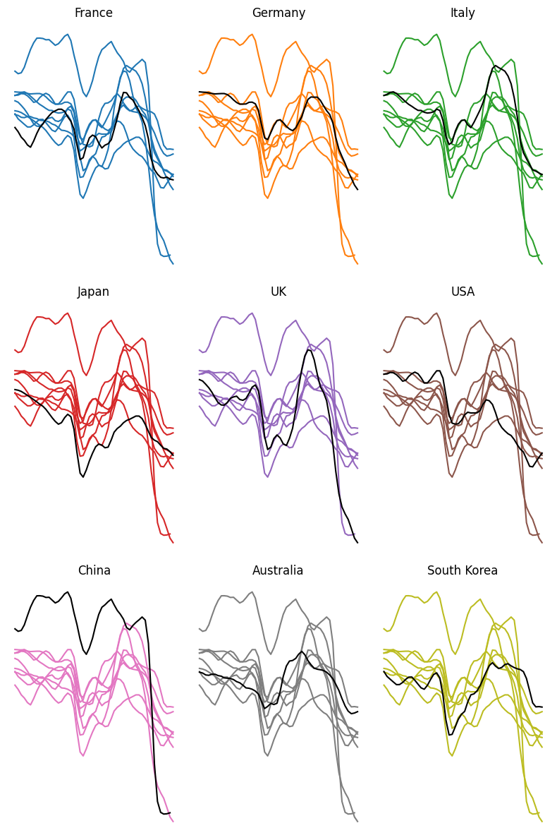
Basic 3x3 line chart with small multiples
We'll start by creating a "simple" graph, with little customization in order to be progressive. Since the final graph is a 3x3 graph, we initialize the sub-graphs with 3 rows and 3 columns. Then, on each sub-plot, we display the same line graph but with different colors.
Only the country of interest will have a fixed color: black. To do this, we iterate over all the distinct categories in the df['country'] variable.
To get a different color for each sub-graph, we use matplotlib's tab10 color map.
For greater readability, we remove most axes and labels. When dealing with small multiples like here, labels on axes can add confusion without being really useful. Later on, we'll add a reference line to help give visibility without adding too much text.
## Create a colormap with a color for each country
num_countries = len(df['country'].unique())
cmap = plt.get_cmap('tab10')

## Init a 3x3 charts
fig, ax = plt.subplots(nrows=3, ncols=3, figsize=(8, 12))

## Plot each group in the subplots
for i, (group, ax) in enumerate(zip(df['country'].unique(), ax.flatten())):

    ## Filter for the group
    filtered_df = df[df['country'] == group]
    other_groups = df['country'].unique()[df['country'].unique() != group]

    ## Plot other groups with lighter colors
    for other_group in other_groups:

        ## Filter observations that are not in the group
        other_y = df['value'][df['country'] == other_group]
        other_x = df['Time'][df['country'] == other_group]

        ## Display the other observations with less opacity.
        ax.plot(other_x, other_y, color=cmap(i))
        ## Sets the opacity for the colors of other groups
        # ax.plot(other_x, other_y, color=cmap(i), alpha=0.2)


    ## Plot the line of the group
    x = filtered_df['Time']
    y = filtered_df['value']
    ax.plot(x, y, color='black')

    ## Removes spines
    ax.spines[['right', 'top', 'left', 'bottom']].set_visible(False)

    ## Remove axis labels
    ax.set_yticks([])
    ax.set_xticks([])

    ## Add a bold title to each subplot
    ax.set_title(f'{group}', fontsize=12)

## Adjust layout and spacing
plt.tight_layout()

## Show the plot
plt.show()
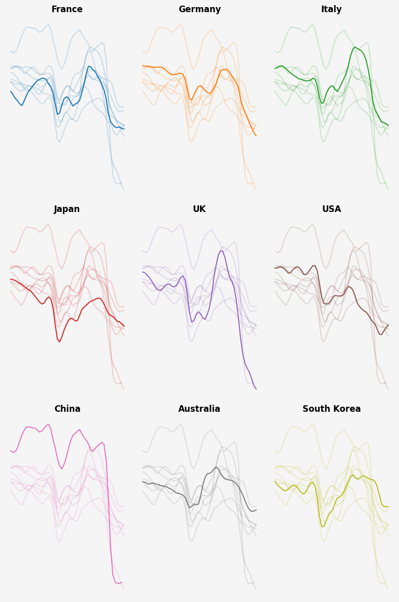
Add an opacity parameter and improve style
As you can see, putting the color of the main country in black does not lead to something very beautiful or easy to read. We want something that showcases the main country while retaining information from other countries, and the answer to this is opacity!.
When we add things in a matplotlib chart, we can change the alpha argument, which is just an opacity argument. In our case, we will just put this parameter lower when plotting the other_group line chart, which is actually very easy.
Also, we change the figure color and background to seashell so that the graphics blend in better than on a white background.
The graph is starting to look really interesting, and gives us a lot of information about consumer confidence in these countries over time!"
## Create a colormap with a color for each country
num_countries = len(df['country'].unique())
cmap = plt.get_cmap('tab10')

## Init a 3x3 charts
fig, ax = plt.subplots(nrows=3, ncols=3, figsize=(8, 12))

## Plot each group in the subplots
for i, (group, ax) in enumerate(zip(df['country'].unique(), ax.flatten())):

    ## Filter for the group
    filtered_df = df[df['country'] == group]
    x = filtered_df['Time']
    y = filtered_df['value']

    ## Set the background color for each subplot: seashell, whitesmoke
    ax.set_facecolor('whitesmoke')
    fig.set_facecolor('whitesmoke')

    ## Plot the line
    ax.plot(x, y, color=cmap(i))

    ## Plot other groups with lighter colors (alpha argument)
    other_groups = df['country'].unique()[df['country'].unique() != group]
    for other_group in other_groups:

        ## Filter observations that are not in the group
        other_y = df['value'][df['country'] == other_group]
        other_x = df['Time'][df['country'] == other_group]

        ## Display the other observations with less opacity (alpha=0.2): sets the opacity for the colors of other groups.
        ax.plot(other_x, other_y, color=cmap(i), alpha=0.2)

    ## Removes spines
    ax.spines[['right', 'top', 'left', 'bottom']].set_visible(False)

    ## Add a bold title to each subplot
    ax.set_title(f'{group}', fontsize=12, fontweight='bold')

    # Remove axis labels
    ax.set_yticks([])
    ax.set_xticks([])

## Adjust layout and spacing
plt.tight_layout()

## Show the plot
plt.show()
Add annotations
Adding annotations is really what takes your graphics to the next level, but it can also be time-consuming. Even if this step adds a lot of lines of code, don't be afraid of it, because there's nothing complicated about it!
In our case, here are the annotations we had :
- Reference line at 100
- Title and description of the metric studied
- Point and value of metric at last date
- Credit and data source
We're mainly using text() function from matplotlib, which makes it super-easy to add text to a graph.
Technical details:
- We use
x - pd.Timedelta(days=300)to place the '100' further to the left (300 days to the left), but as the x-axis is in datetime format, we can't use only integers. - The position of the reference lines is calculated so that it starts at the first available date and ends at the last available date. To do this, we sort the data frame and obtain the first and last rows.
- The credit positions are determined through trial and error (i.e. I tried different positions until I found the right one).
## Create a colormap with a color for each country
num_countries = len(df['country'].unique())
cmap = plt.get_cmap('tab10')

## Init a 3x3 charts
fig, ax = plt.subplots(nrows=3, ncols=3, figsize=(8, 12))

## Add a big title on top of the entire chart
fig.suptitle('\nConsumer \nConfidence \naround the \nWorld\n\n', ## Title ('\n' allows you to go to the line),
             fontsize=40,
             fontweight='bold',
             x=0.05,   ## Shift the text to the left
             ha='left' ## Align the text to the left
            )

## Add a paragraph of text on the right of the title
paragraph_text = (
    "The consumer confidence indicator\n"
    "provided an indication of future\n"
    "developments of households'.\n"
    "consumption and saving. An\n"
    "indicator above 100 signals a boost\n"
    "in the consumers' confidence\n"
    "towards the future economic\n"
    "situation. Values below 100 indicate\n"
    "a pessimistic attitude towards future\n"
    "developments in the economy,\n"
    "possibly resulting in a tendency to\n"
    "save more and consume less. During\n"
    "2022, the consuer confidence\n"
    "indicators have declined in many\n"
    "major economies around the world.\n"
)
fig.text(0.5, 0.92,      ## Position
         paragraph_text, ## Content
         fontsize=12,
         va='top',  ## Put the paragraph at the top of the chart
         ha='left', ## Align the text to the left
        )

## Plot each group in the subplots
for i, (group, ax) in enumerate(zip(df['country'].unique(), ax.flatten())):

    ## Filter for the group
    filtered_df = df[df['country'] == group]
    x = filtered_df['Time']
    y = filtered_df['value']

    ## Get last value (according to 'Time') for the group
    sorted_df  = filtered_df.sort_values(by='Time')
    last_value = sorted_df.iloc[-1]['value']
    last_date  = sorted_df.iloc[-1]['Time']

    ## Set the background color for each subplot: seashell, whitesmoke
    ax.set_facecolor('whitesmoke')
    fig.set_facecolor('whitesmoke')

    ## Plot the line
    ax.plot(x, y, color=cmap(i))

    ## Add the final value
    ax.plot(last_date,     ## x-axis position
            last_value,    ## y-axis position
            marker='o',    ## Style of the point
            markersize=5,  ## Size of the point
            color=cmap(i), ## Color
           )

    ## Add the text of the value
    ax.text(last_date,
             last_value*1.005,       ## slightly shift up
             f'{round(last_value)}', ## round for more lisibility
             fontsize=7,
             color=cmap(i),          ## color
             fontweight='bold',
           )

    ## Add the 100 on the left
    ax.text(sorted_df.iloc[0]['Time'] - pd.Timedelta(days=300), ## shift the position to the left
             100,
             '100',
             fontsize=10,
             color='black',)

    ## Add line
    sorted_df = df.sort_values(by='Time')
    start_x_position = sorted_df.iloc[0]['Time']
    end_x_position = sorted_df.iloc[-1]['Time']
    ax.plot([start_x_position, end_x_position], ## x-axis position
            [100, 100],                         ## y-axis position (constant position)
            color='black',                      ## Color
            alpha=0.8,                          ## Opacity
            linewidth=0.8,                      ## Width of the line
           )

    ## Plot other groups with lighter colors (alpha argument)
    other_groups = df['country'].unique()[df['country'].unique() != group]
    for other_group in other_groups:

        ## Filter observations that are not in the group
        other_y = df['value'][df['country'] == other_group]
        other_x = df['Time'][df['country'] == other_group]

        ## Display the other observations with less opacity (alpha=0.2)
        ax.plot(other_x, other_y, color=cmap(i), alpha=0.2)

    ## Removes spines
    ax.spines[['right', 'top', 'left', 'bottom']].set_visible(False)

    ## Add a bold title to each subplot
    ax.set_title(f'{group}', fontsize=12, fontweight='bold')

    ## Customizing x-axis for years 2019, 2020, 2021, 2022
    ax.grid(True)     ## Enable grid

    year_labels = ['19', '20', '21', '22']  ## Labels for years 2019, 2020, 2021, 2022
    year_positions = [pd.Timestamp(f'{year}-01-01') for year in range(2019, 2023)]  ## Position for each year label
    ## Display x-axis labels only for the last row (3rd row in 3x3)
    ax.set_yticklabels([])           ## Hide y-axis lables
    ax.set_xticks(year_positions)    ## Set x-axis custom ticks
    if i // 3 == 2:  ## Check if the subplot is in the third row (indexing starts at 0)
        ax.set_xticklabels(year_labels)   ## Set custom x-axis labels for years
    else:
        ax.set_xticklabels([])            ## Hide x-axis ticks labels


## Add a credit section at the bottom of the chart
fig.text(0.0, -0.025,  ## position
         "Data:",      ## text
         fontsize=10,
         va='bottom',
         ha='left',
         fontweight='bold',)
fig.text(0.07, -0.025, ## position
         "OECD, 2022",
         fontsize=10,
         va='bottom',
         ha='left')

## Adjust layout and spacing
plt.tight_layout()

## Show the plot
plt.show()
Next Steps
-
This page showcases the work of Gilbert Fontana, initially published in the Visual Capitalist.
- The chart was originally made with R. This post is a translation to Python by Joseph B..
- This article explains how to reproduce a line chart with small multiples, originally design by Gilbert Fontana.
-
For more examples of advanced customization, check out this other reproduction of Fontana's work. Also, you might be interested in adding an image/logo to your chart.