Correlogram with Seaborn
This post aims to explain how to improve it. It is divided in 2 parts: how to custom the correlation observation (for each pair of numeric variable), and how to custom the distribution (diagonal of the matrix).
Correlation
The seaborn library allows to draw a correlation matrix through the pairplot() function. The parameters to create the example graphs are:
data: dataframekind: kind of plot to make (possible kinds are ‘scatter’, ‘kde’, ‘hist’, ‘reg’)
# !pip install seaborn
# library & dataset
import matplotlib.pyplot as plt
import seaborn as sns
df = sns.load_dataset('iris')
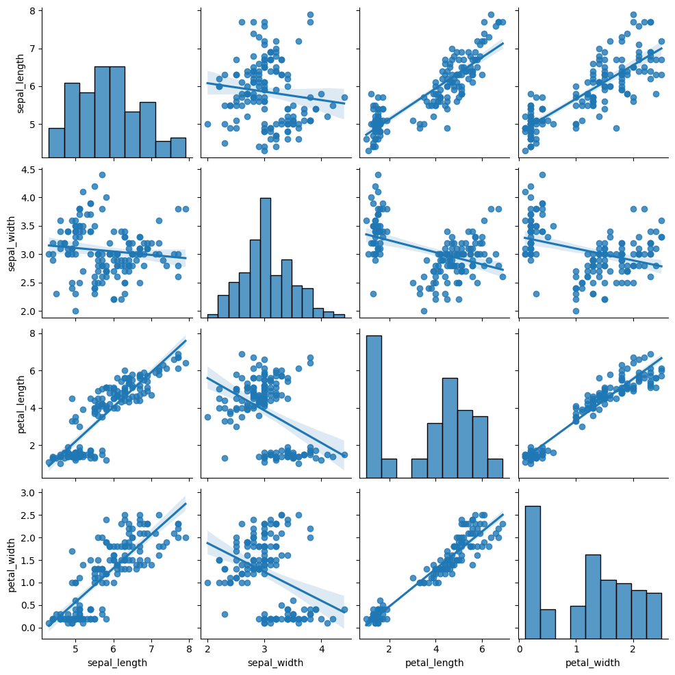
# with regression
sns.pairplot(df, kind="reg")
plt.show()
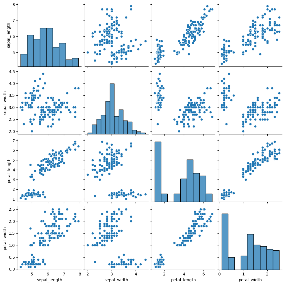
# without regression
sns.pairplot(df, kind="scatter")
plt.show()
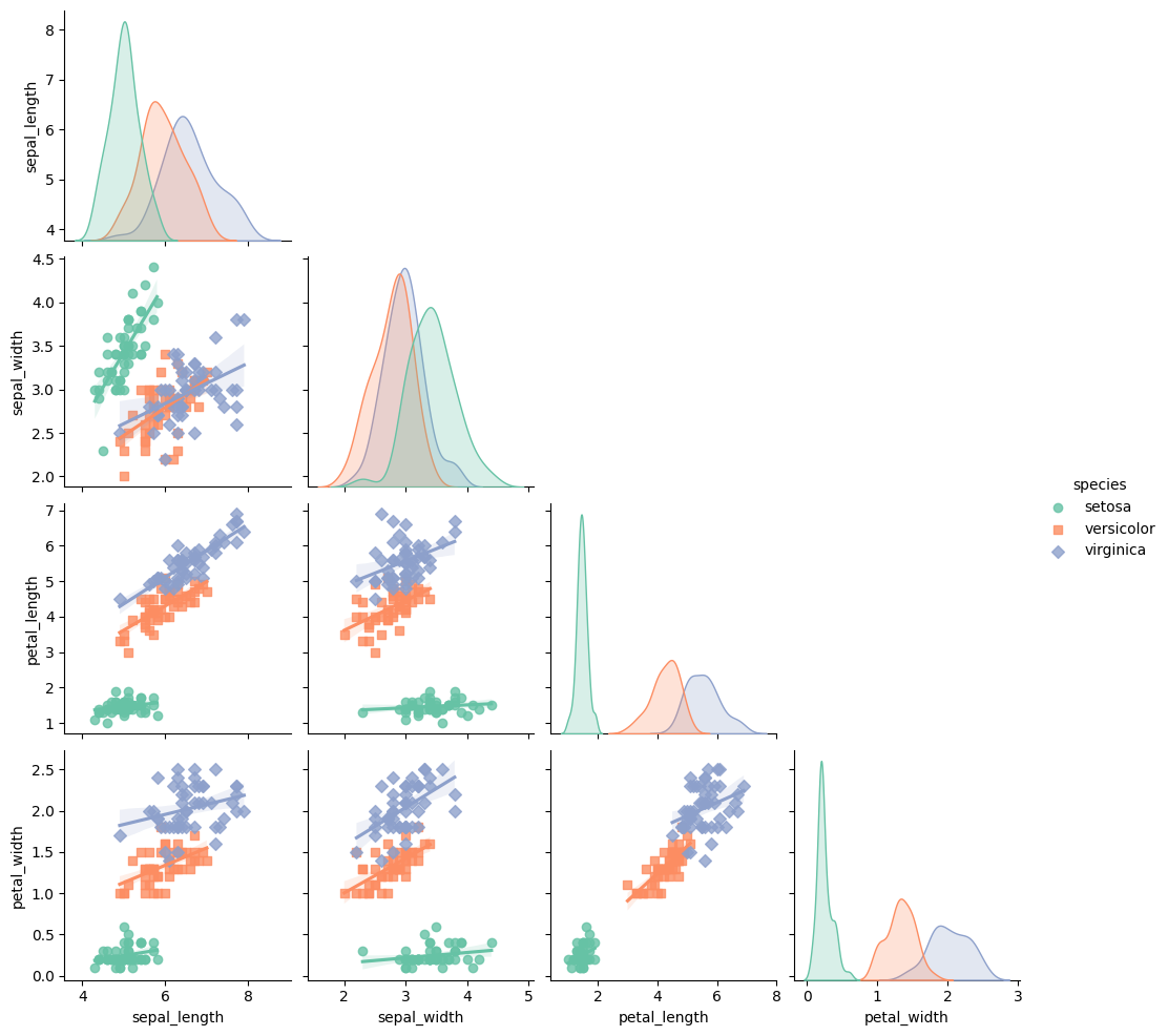
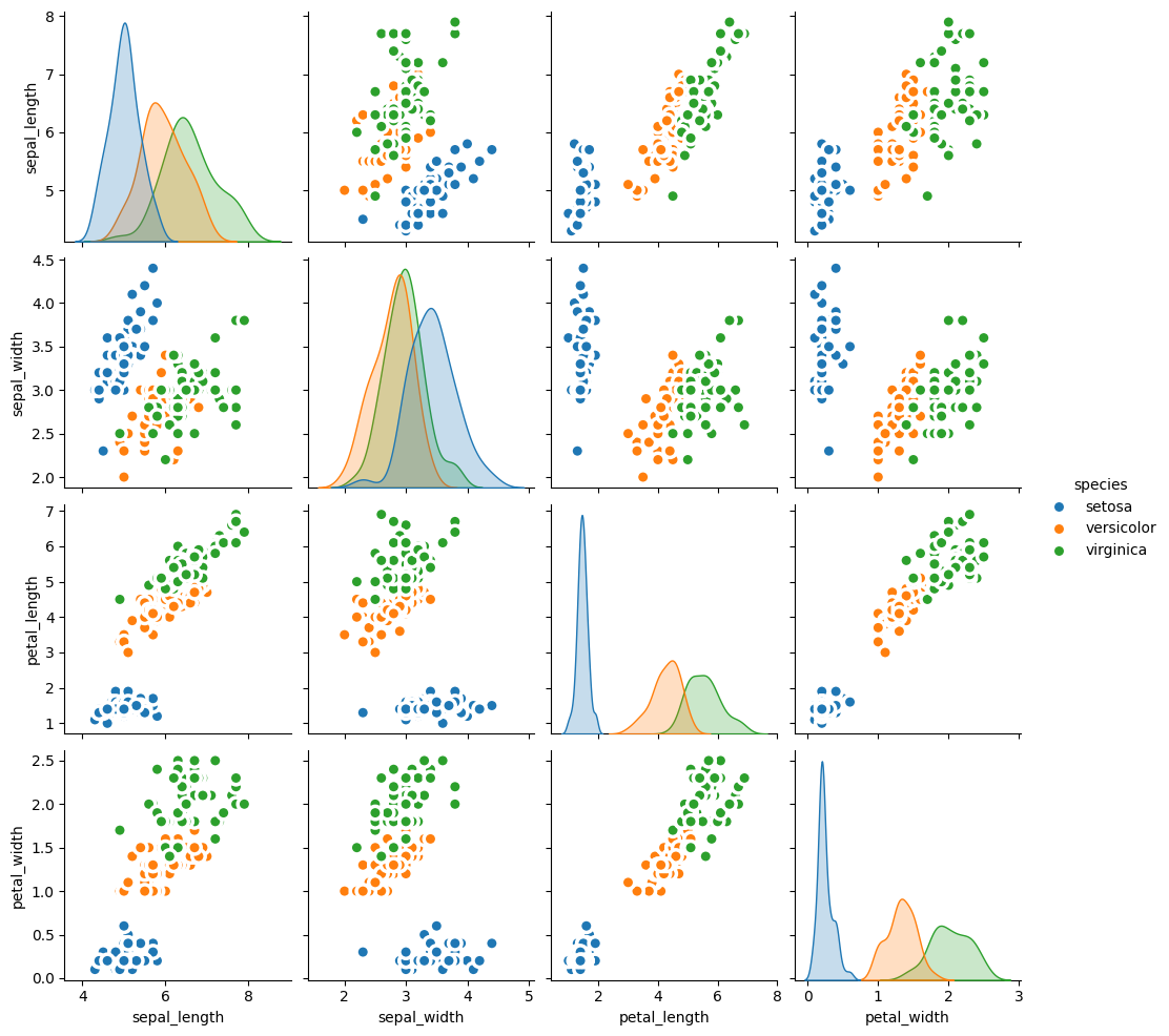
In a graph drawn by pairplot() function of seaborn, you can control the marker features, colors and data groups by using additional parameters such as:
hue: variables that define subsets of the datamarkers: a list of marker shapespalette: set of colors for mapping the hue variableplot_kws: a dictionary of keyword arguments to modificate the plot
## library & dataset
import matplotlib.pyplot as plt
import seaborn as sns
df = sns.load_dataset('iris')
## Left/top
# sns.pairplot(df, kind="scatter", hue="species", markers=["o", "s", "D"], palette="Set2")
## Create the pairplot
pair_plot = sns.pairplot(df, kind="reg", hue="species", markers=["o", "s", "D"], palette="Set2")
## Iterate through axes to remove upper triangle
for i in range(len(df.columns) - 1):
for j in range(i + 1, len(df.columns) - 1):
pair_plot.axes[i, j].remove()
plt.show()
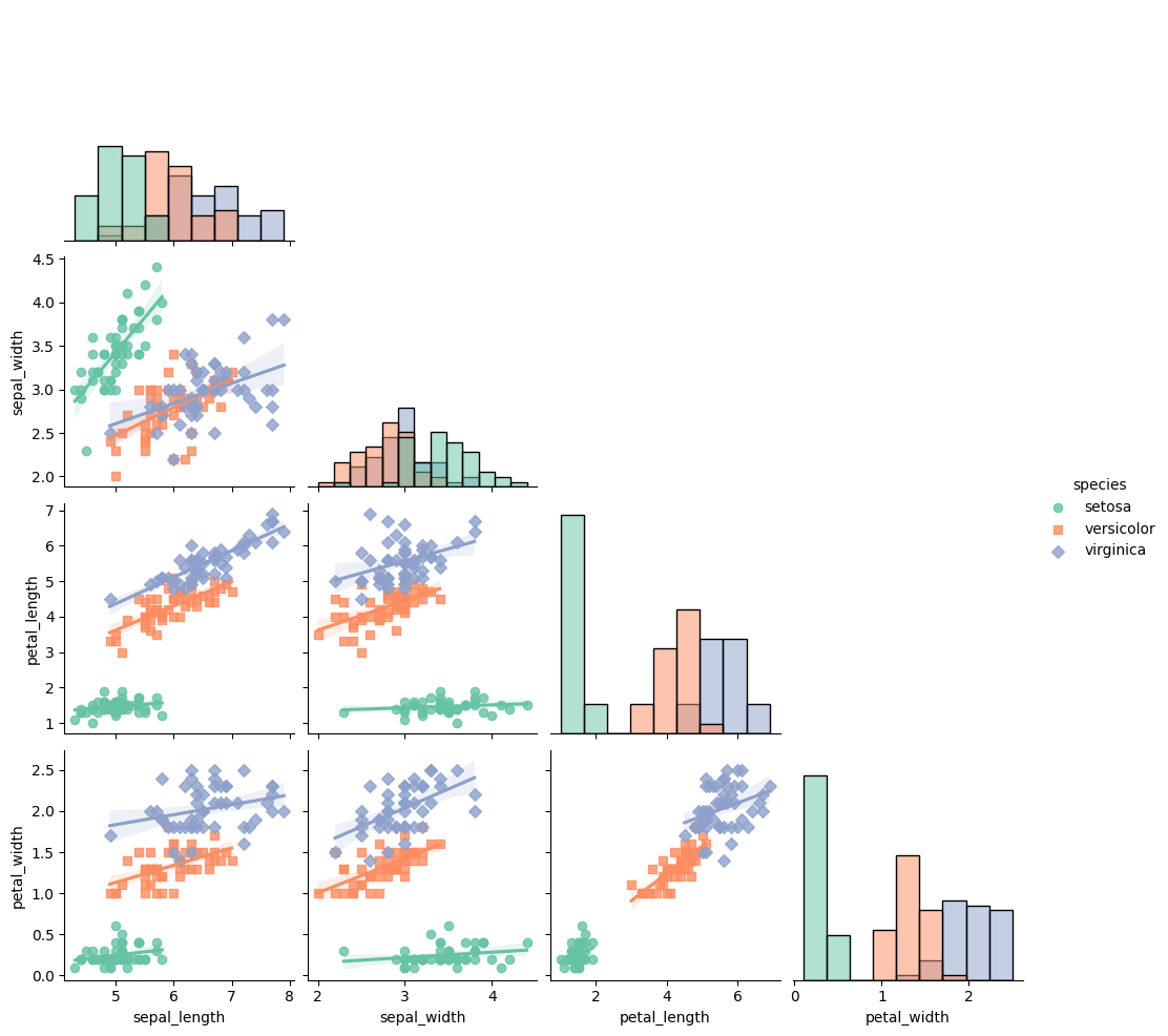
## Right/Bottom
# sns.pairplot(df, kind="scatter", hue="species", markers=["o", "s", "D"], palette="Set2")
## Create the pairplot
pair_plot = sns.pairplot(df, kind="reg", diag_kind='hist', hue="species", markers=["o", "s", "D"], palette="Set2", corner = True)
plt.show()
## library & dataset
# import matplotlib.pyplot as plt
# import seaborn as sns
# df = sns.load_dataset('iris')

## Right/bottom: you can give other arguments with plot_kws.
sns.pairplot(df, kind="scatter", hue="species", plot_kws=dict(s=80, edgecolor="white", linewidth=2.5))
plt.show()
Distribution
As you can select the kind of plot to make in pairplot() function, you can also select the kind of plot for the diagonal subplots.
diag_kind: the kind of plot for the diagonal subplots (possible kinds are ‘auto’, ‘hist’, ‘kde’, None)
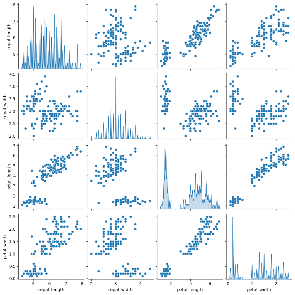
Note that you can use bw_adjust to increase or decrease the amount of smoothing.
# library & dataset
import seaborn as sns
import matplotlib.pyplot as plt
# Load dataset
df = sns.load_dataset('iris')
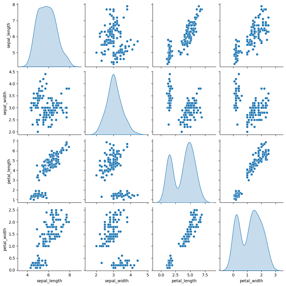
# Density
sns.pairplot(df, diag_kind="kde")
# sns.pairplot(df, diag_kind="kde", diag_kws=dict(fill=True, bw_adjust=.05))
# Histogram
sns.pairplot(df, diag_kind="hist")
# You can custom it as a density plot or histogram so see the related sections
# sns.pairplot(df, diag_kind="kde", diag_kws=dict(shade=True, bw_adjust=.05, vertical=False) )
# Ensure that 'fill' is used in all density plot configurations
sns.pairplot(df, diag_kind="kde", diag_kws=dict(fill=True, bw_adjust=.05))
plt.show()

References
The post shows how to make a basic correlogram with seaborn.